As a quick recap, in the last post the primary focus was introducing how images are processed to create the feature vectors, and how the logistic regression model is used to predict $$\hat y$$. In addition, the concept of loss function:

$$L(\hat y\ ,\ y)\ =\ -(y\ \log\ \hat y\ +\ (1\ -\ y)\ \log\ (1-\ \hat y))$$

was introduced to measure how well that prediction was on a single training example, while the cost function:

$$J(w,b)\ =\ {{1}\over{m}}\sum\limits_{i\ =\ 1}^{m}{L({\hat y}^{(i)}\ ,\ y^{(i)})\ }\ =\ \ -\ {{1}\over{m}}\sum\limits_{i\ =\ 1}^{m}{[y^{(i)}\ \log\ {\hat y}^{^{(i)}}\ +\ (1\ -\ y^{^{(i)}})\ \log\ (1-\ {\hat y}^{^{(i)}})]\ }$$

is used to determine how well the parameters w and b work across the entire data set (m). As it turns out, the cost function is a convex function, meaning that it has only one local minimum optima, and finding the values of w and b that minimize this cost function is the objective, and this minimum value corresponds to the global optimum as depicted in Figure 1 below:

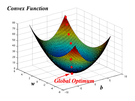
Obtaining this global optimum is derived by using the gradient descent.

Gradient Descent:

To obtain the values for w and b that give us the global optimum we initialize the values w and bto some value that corresponds to the red dot in Figure 1. As we cycle through the layers of the neural network, the logistic model is adjusted by changing w and b and this adjustment is called the “learning rate” alpha ($$\alpha$$) which moves the calculated values of the cost function closer and closer to the global optimum.

As you recall from calculus, the derivative of a function is the slope of the function at a given point.  So w and b are updated with each iteration with the following formulas:

$$w:=\ w\ -\ \alpha\ {{\partial\ J(w,\ b)}\over{\partial w}}$$

$$b\ :=\ b\ -\ \alpha\ {{\partial\ J(w,\ b)}\over{\partial b}}$$

Taking the partial derivative of J(w,b) with respect to w and J(w,b) with respect to b. What happens is that if the partial derivative with respect to wis negative, then the value of w is increased, because a negative minus a negative is positive, and likewise, if the value of the partial derivative is positive, then the value of w is decreased. As the algorithm continues, the values get closer and closer to the global minimum. Obviously, when the partial derivative is 0, parameters are at their optimal value.

Computation Graph:

This section introduces the key equations needed to implement gradient descent for logistic regression using a computation graph. Logistic regression is as follows:

$$z^{[l]}\ \ =\ w^{[l]}\ x\ +\ b^{[l]}$$

$$\hat y\ =\ a^{(i)}\ =\ \sigma (z^{(i)})$$

$$L(\hat y\ ,\ y)\ =\ -(y\ \log\ \hat y\ +\ (1\ -\ y)\ \log\ (1-\ \hat y))$$

For the loss function, we will replace $$\hat y$$ with a and y is the actual value for the image (1 = dog, 0 = no dog), so we are left with:

$$L(a\ ,\ y)\ =\ -(y\ \log\ a\ +\ (1\ -\ y)\ \log\ (1-\ a))$$

At this point we will write this as a computation graph, and use an example where we have two feature values:

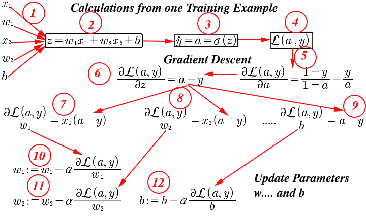
1. Feature input vector x with initialized values for w and b.
2. Calculate the zvalue using logistic regression
3. With the output from $$\sigma\ (z)$$,  $$\hat y$$ is calculated
4. The loss function is calculated using a
5. The derivative of the loss function is calculated
6. The derivative of the loss function with respect to z is calculated, which reduces to a - y.
7. The derivative of the loss function with respect to w1 is calculated — abbreviated dwin the code
8. The derivative of the loss function with respect to w2 is calculated — abbreviated dwin the code
9. The derivative of the loss function with respect to b is calculated — abbreviated dbin the code
10. The parameter w1 is updated
11. The parameter w2 is updated
12. The parameter b is updated

Now that we see how to calculate gradient descent for one training example (one image), we will look at calculating it for an entire training set of m training examples.

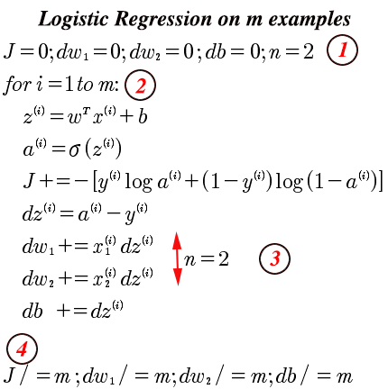
1. Initialize variables, again this is an example with 2 input feature values. Just one image with dimensions of 250 x 250 x 3 has 187,500 feature values per example, so this example would require a for loop that would be impractical without vectorizing the images and being able to do vector operations.
2. m represents the number of images in the training set. This could 1 or 1,000.
3. For n = 2this algorithm is adequate, but requires a forloop to process 187,500 n values. This would not be efficient, and requires vectorization which will be explained in the code section.
4. After looping through each image, we still need to divide the values by m to get the averages. J would be the cost function.

Building a Deep Neural Network:

The following provides guidance for building all of the functions required for a deep neural network. Following this we will use these functions to build a deep neural network for image classification.

The process goes as follows (from deeplearning.ai – Coursera “Neural Networks and Deep Learning”):

1. Initialize the parameters for a two-layer network and for an $$L$$-layer neural network.
2. Implement the forward propagation module (shown in purple in the figure below).
   1. Complete the LINEAR part of a layer’s forward propagation step (resulting in $$Z^{[l]}$$).
   2. Apply the ACTIVATION function (relu/sigmoid).
   3. Combine the previous two steps into a new [LINEAR->ACTIVATION] forward function.
   4. Stack the [LINEAR->RELU] forward function L-1 time (for layers 1 through L-1) and add a [LINEAR->SIGMOID] at the end (for the final layer $L$). This gives you a new L_model_forward function.
3. Compute the loss.
4. Implement the backward propagation module (denoted in red in the figure below).
   1. Complete the LINEAR part of a layer’s backward propagation step.
   2. Compute the gradient of the ACTIVATION function (relu_backward/sigmoid_backward)
   3. Combine the previous two steps into a new [LINEAR->ACTIVATION] backward function.
   4. Stack [LINEAR->RELU] backward L-1 times and add [LINEAR->SIGMOID] backward in a new L_model_backward function
5. Finally update the parameters.
   

   Figure 1: Deep Learning Neural Network

An important point here is that for every forward function, there is a corresponding backward function. As you step through the forward model, at each step you cache the $$Z^{[l]}$$ value to be used during the backward propagation to compute gradients.